10 Minutes to DeepGraph¶

[ipython notebook] [python script] [data]

This is a short introduction to DeepGraph. In the following, we demonstrate DeepGraph’s core functionalities by a toy data-set, “flying balls”.

First of all, we need to import some packages

# for plots
import matplotlib.pyplot as plt

# the usual
import numpy as np
import pandas as pd

import deepgraph as dg

# notebook display
%matplotlib inline
plt.rcParams['figure.figsize'] = 8, 6
pd.options.display.max_rows = 10
pd.set_option('expand_frame_repr', False)

Loading Toy Data

Then, we need data in the form of a pandas DataFrame, representing the nodes of our graph

v = pd.read_csv('flying_balls.csv', index_col=0)
print(v)

      time            x          y  ball_id
      0  1692.000000   0.000000        0
      0  8681.000000   0.000000        1
      0   490.000000   0.000000        2
      0  7439.000000   0.000000        3
      0  4998.000000   0.000000        4
...    ...          ...        ...      ...
  45  2812.552734  16.503178       39
  46  5686.915998  14.161693       10
  46  3161.729086  19.381823       14
  46  5594.233413  57.701712       37
  47  5572.216748  20.588750       37

[1168 rows x 4 columns]

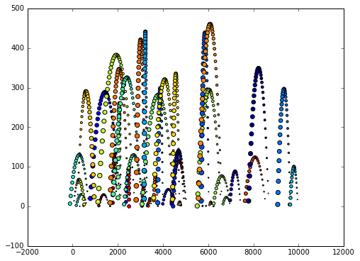
The data consists of 1168 space-time measurements of 50 different toy balls in two-dimensional space. Each space-time measurement (i.e. row of v) represents a node.

Let’s plot the data such that each ball has it’s own color

plt.scatter(v.x, v.y, s=v.time, c=v.ball_id)

Creating Edges¶

In order to create edges between these nodes, we now initiate a dg.DeepGraph instance

g = dg.DeepGraph(v)
g

<DeepGraph object, with n=1168 node(s) and m=0 edge(s) at 0x7facf3b35dd8>

and use it to create edges between the nodes given by g.v. For that matter, we may define a connector function

def x_dist(x_s, x_t):
    dx = x_t - x_s
    return dx

and pass it to g.create_edges in order to compute the distance in the x-coordinate of each pair of nodes

g.create_edges(connectors=x_dist)
g

<DeepGraph object, with n=1168 node(s) and m=681528 edge(s) at 0x7facf3b35dd8>

print(g.e)

                    dx
s    t
  1     6989.000000
  -1202.000000
   5747.000000
   3306.000000
   2812.000000
...                ...
1166   -92.682585
-114.699250
1166  2432.504327
2410.487662
1167   -22.016665

[681528 rows x 1 columns]

Let’s say we’re only interested in creating edges between nodes with a x-distance smaller than 1000. Then we may additionally define a selector

def x_dist_selector(dx, sources, targets):
    dxa = np.abs(dx)
    sources = sources[dxa <= 1000]
    targets = targets[dxa <= 1000]
    return sources, targets

and pass both the connector and selector to g.create_edges

g.create_edges(connectors=x_dist, selectors=x_dist_selector)
g

<DeepGraph object, with n=1168 node(s) and m=156938 edge(s) at 0x7facf3b35dd8>

print(g.e)

                   dx
s    t
  6     416.000000
   848.000000
 -973.000000
  437.000000
  778.000000
...               ...
1167  -44.033330
1165  349.176351
1166  -92.682585
-114.699250
1167  -22.016665

[156938 rows x 1 columns]

There is, however, a much more efficient way of creating edges that involve a simple distance threshold such as the one above

Creating Edges on a FastTrack¶

In order to efficiently create edges including a selection of edges via a simple distance threshold as above, one should use the create_edges_ft method. It relies on a sorted DataFrame, so we need to sort g.v first

g.v.sort_values('x', inplace=True)

g.create_edges_ft(ft_feature=('x', 1000))
g

<DeepGraph object, with n=1168 node(s) and m=156938 edge(s) at 0x7facf3b35dd8>

Let’s compare the efficiency

%timeit -n3 -r3 g.create_edges(connectors=x_dist, selectors=x_dist_selector)

3 loops, best of 3: 557 ms per loop

%timeit -n3 -r3 g.create_edges_ft(ft_feature=('x', 1000))

3 loops, best of 3: 167 ms per loop

The create_edges_ft method also accepts connectors and selectors as input. Let’s connect only those measurements that are close in space and time

def y_dist(y_s, y_t):
    dy = y_t - y_s
    return dy

def time_dist(time_t, time_s):
    dt = time_t - time_s
    return dt

def y_dist_selector(dy, sources, targets):
    dya = np.abs(dy)
    sources = sources[dya <= 100]
    targets = targets[dya <= 100]
    return sources, targets

def time_dist_selector(dt, sources, targets):
    dta = np.abs(dt)
    sources = sources[dta <= 1]
    targets = targets[dta <= 1]
    return sources, targets

g.create_edges_ft(ft_feature=('x', 100),
                  connectors=[y_dist, time_dist],
                  selectors=[y_dist_selector, time_dist_selector])
g

<DeepGraph object, with n=1168 node(s) and m=1899 edge(s) at 0x7facf3b35dd8>

print(g.e)

         dt         dy       ft_r
s   t
867  -1  19.311136  33.415831
843  -1  17.678482  33.415831
818  -1  16.045829  33.415831
792  -1  14.413176  33.415831
766  -1  12.780523  33.415831
...      ..        ...        ...
203  -1 -10.825226  15.455612
159  -1 -12.457879  15.455612
114  -1 -14.090532  15.455612
65   -1 -15.723185  15.455612
16   -1 -17.355838  15.455612

[1899 rows x 3 columns]

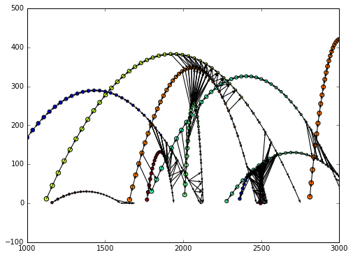
We can now plot the flying balls and the edges we just created with the plot_2d method

obj = g.plot_2d('x', 'y', edges=True,
                kwds_scatter={'c': g.v.ball_id, 's': g.v.time})
obj['ax'].set_xlim(1000,3000)

Graph Partitioning¶

The DeepGraph class also offers methods to partition nodes, edges and an entire graph. See the docstrings and the other tutorials for details and examples.

Graph Interfaces¶

Furthermore, you may inspect the docstrings of return_cs_graph, return_nx_graph and return_gt_graph to see how to convert from DeepGraph’s DataFrame representation of a network to sparse adjacency matrices, NetworkX’s network representation and graph_tool’s network representation.

Plotting Methods¶

DeepGraph also offers a number of useful Plotting methods. See plotting methods for details and have a look at the other tutorials for examples.